WHR (2017): Principal Component Analysis
Introduction
The first World Happiness Report was published in April, 2012, in support of the UN High Level Meeting on happiness and well-being. Since then the world has come a long way. Increasingly, happiness is considered to be the proper measure of social progress and the goal of public policy. In June 2016 the OECD committed itself “to redefine the growth narrative to put people’s well-being at the center of governments’ efforts”. In February 2017, the United Arab Emirates held a full-day World Happiness meeting, as part of the World Government Summit. Now on World Happiness Day, March 20th, we launch the World Happiness Report 2017, once again back at the United Nations, again published by the Sustainable Development Solutions Network, and now supported by a generous three-year grant from the Ernesto Illy Foundation.
- Report link:
 http://worldhappiness.report/
Objectif
Find a relationship between the variable “country” and other indicators to understand the factors of the general trend of happiness.
Import necessary packages
library(FactoMineR)
library(factoextra)
## Loading required package: ggplot2
## Welcome! Related Books: `Practical Guide To Cluster Analysis in R` at https://goo.gl/13EFCZ
library(ggplot2)
library(summarytools)
Import Data
Happy = read.csv("data/principal_component_analysis/2017.csv")
head(Happy)
##       Country Happiness.Rank Happiness.Score Whisker.high Whisker.low
## 1      Norway              1           7.537     7.594445    7.479556
## 2     Denmark              2           7.522     7.581728    7.462272
## 3     Iceland              3           7.504     7.622030    7.385970
## 4 Switzerland              4           7.494     7.561772    7.426227
## 5     Finland              5           7.469     7.527542    7.410458
## 6 Netherlands              6           7.377     7.427426    7.326574
##   Economy..GDP.per.Capita.   Family Health..Life.Expectancy.   Freedom
## 1                 1.616463 1.533524                0.7966665 0.6354226
## 2                 1.482383 1.551122                0.7925655 0.6260067
## 3                 1.480633 1.610574                0.8335521 0.6271626
## 4                 1.564980 1.516912                0.8581313 0.6200706
## 5                 1.443572 1.540247                0.8091577 0.6179509
## 6                 1.503945 1.428939                0.8106961 0.5853845
##   Generosity Trust..Government.Corruption. Dystopia.Residual
## 1  0.3620122                     0.3159638          2.277027
## 2  0.3552805                     0.4007701          2.313707
## 3  0.4755402                     0.1535266          2.322715
## 4  0.2905493                     0.3670073          2.276716
## 5  0.2454828                     0.3826115          2.430182
## 6  0.4704898                     0.2826618          2.294804
Add Region Column (Python Code)
import pandas as pd
from hdx.location.country import Country
df = pd.read_csv("2017.csv")
regions = []
for i in range(len(df)):
    country = df.Country[i]
    code = Country.get_iso3_country_code_fuzzy(country)[0]
    info = Country.get_country_info_from_iso3(code)
    region = info['Sub-region Name']
    regions.append(region)
df['Region'] = regions
Happy = read.csv("data/principal_component_analysis/data_2017.csv")
rownames(Happy) = Happy$Country
Happy = Happy[c("Region","Happiness.Score","Whisker.high","Whisker.low","Economy..GDP.per.Capita.","Family","Health..Life.Expectancy.","Freedom","Generosity","Trust..Government.Corruption.","Dystopia.Residual")]
attach(Happy)
head(Happy)
##                      Region Happiness.Score Whisker.high Whisker.low
## Norway      Northern Europe           7.537     7.594445    7.479556
## Denmark     Northern Europe           7.522     7.581728    7.462272
## Iceland     Northern Europe           7.504     7.622030    7.385970
## Switzerland  Western Europe           7.494     7.561772    7.426227
## Finland     Northern Europe           7.469     7.527542    7.410458
## Netherlands  Western Europe           7.377     7.427426    7.326574
##             Economy..GDP.per.Capita.   Family Health..Life.Expectancy.
## Norway                      1.616463 1.533524                0.7966665
## Denmark                     1.482383 1.551122                0.7925655
## Iceland                     1.480633 1.610574                0.8335521
## Switzerland                 1.564980 1.516912                0.8581313
## Finland                     1.443572 1.540247                0.8091577
## Netherlands                 1.503945 1.428939                0.8106961
##               Freedom Generosity Trust..Government.Corruption.
## Norway      0.6354226  0.3620122                     0.3159638
## Denmark     0.6260067  0.3552805                     0.4007701
## Iceland     0.6271626  0.4755402                     0.1535266
## Switzerland 0.6200706  0.2905493                     0.3670073
## Finland     0.6179509  0.2454828                     0.3826115
## Netherlands 0.5853845  0.4704898                     0.2826618
##             Dystopia.Residual
## Norway               2.277027
## Denmark              2.313707
## Iceland              2.322715
## Switzerland          2.276716
## Finland              2.430182
## Netherlands          2.294804
Descriptive statistics
dfSummary(Happy)
## Data Frame Summary
## Happy
## N: 155
## --------------------------------------------------------------------------------------------------------------------------------------------------
## No   Variable                         Stats / Values                   Freqs (% of Valid)    Text Graph                         Valid    Missing
## ---- -------------------------------- -------------------------------- --------------------- ---------------------------------- -------- ---------
## 1    Region                           1. Australia and New Zealand      2 ( 1.3%)                                               155      0
##      [factor]                         2. Central Asia                   5 ( 3.2%)            I                                  (100%)   (0%)
##                                       3. Eastern Asia                   6 ( 3.9%)            I
##                                       4. Eastern Europe                10 ( 6.5%)            II
##                                       5. Latin America and the Car     22 (14.2%)            IIII
##                                       6. Northern Africa                6 ( 3.9%)            I
##                                       7. Northern America               2 ( 1.3%)
##                                       8. Northern Europe               10 ( 6.5%)            II
##                                       9. South-eastern Asia             8 ( 5.2%)            I
##                                       10. Southern Asia                 8 ( 5.2%)            I
##                                       [ 4 others ]                     76 (49.0%)            IIIIIIIIIIIIIIII
##
## 2    Happiness.Score                  mean (sd) : 5.35 (1.13)          151 distinct values             : .                      155      0
##      [numeric]                        min < med < max :                                            .   : :                      (100%)   (0%)
##                                       2.69 < 5.28 < 7.54                                         . : : : : : .
##                                       IQR (CV) : 1.6 (0.21)                                    : : : : : : : : :
##                                                                                              . : : : : : : : : :
##
## 3    Whisker.high                     mean (sd) : 5.45 (1.12)          155 distinct values             : .                      155      0
##      [numeric]                        min < med < max :                                                : :                      (100%)   (0%)
##                                       2.86 < 5.37 < 7.62                                         . : : : : . .
##                                       IQR (CV) : 1.59 (0.21)                                   : : : : : : : : :
##                                                                                              . : : : : : : : : :
##
## 4    Whisker.low                      mean (sd) : 5.26 (1.15)          155 distinct values             : .                      155      0
##      [numeric]                        min < med < max :                                            .   : :                      (100%)   (0%)
##                                       2.52 < 5.19 < 7.48                                         . : : : : . .
##                                       IQR (CV) : 1.63 (0.22)                                   . : : : : : : : :
##                                                                                              . : : : : : : : : :
##
## 5    Economy..GDP.per.Capita.         mean (sd) : 0.98 (0.42)          155 distinct values             .   :                    155      0
##      [numeric]                        min < med < max :                                                : : :                    (100%)   (0%)
##                                       0 < 1.06 < 1.87                                              . : : : :
##                                       IQR (CV) : 0.65 (0.43)                                   : : : : : : : .
##                                                                                              : : : : : : : : : .
##
## 6    Family                           mean (sd) : 1.19 (0.29)          155 distinct values               : .                    155      0
##      [numeric]                        min < med < max :                                                  : :                    (100%)   (0%)
##                                       0 < 1.25 < 1.61                                                  : : :
##                                       IQR (CV) : 0.37 (0.24)                                         : : : :
##                                                                                                  . : : : : :
##
## 7    Health..Life.Expectancy.         mean (sd) : 0.55 (0.24)          155 distinct values               :                      155      0
##      [numeric]                        min < med < max :                                                  :   :                  (100%)   (0%)
##                                       0 < 0.61 < 0.95                                                  . : : :
##                                       IQR (CV) : 0.35 (0.43)                                     . : . : : : :
##                                                                                              : : : : : : : : : :
##
## 8    Freedom                          mean (sd) : 0.41 (0.15)          155 distinct values           :                          155      0
##      [numeric]                        min < med < max :                                              : .                        (100%)   (0%)
##                                       0 < 0.44 < 0.66                                            . . : :
##                                       IQR (CV) : 0.21 (0.37)                                     : : : : .
##                                                                                              . : : : : : :
##
## 9    Generosity                       mean (sd) : 0.25 (0.13)          155 distinct values       :                              155      0
##      [numeric]                        min < med < max :                                        . :                              (100%)   (0%)
##                                       0 < 0.23 < 0.84                                          : : .
##                                       IQR (CV) : 0.17 (0.55)                                 : : : : .
##                                                                                              : : : : : .
##
## 10   Trust..Government.Corruption.    mean (sd) : 0.12 (0.1)           155 distinct values     :                                155      0
##      [numeric]                        min < med < max :                                        :                                (100%)   (0%)
##                                       0 < 0.09 < 0.46                                        : : :
##                                       IQR (CV) : 0.1 (0.83)                                  : : : .
##                                                                                              : : : : . : :   . .
##
## 11   Dystopia.Residual                mean (sd) : 1.85 (0.5)           155 distinct values         :                            155      0
##      [numeric]                        min < med < max :                                            :                            (100%)   (0%)
##                                       0.38 < 1.83 < 3.12                                           : :
##                                       IQR (CV) : 0.55 (0.27)                                     . : :
##                                                                                                . : : : :
## ---------------------------------------------------------------------------------------------------------------------------------
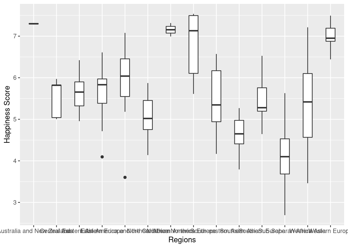
Boxplot
ggplot(Happy, aes(Region,Happiness.Score))+
  geom_boxplot(width=0.4) +
  ylab('Happiness Score') +
  xlab('Regions')
Scree Plot
- The elbow effect appears from the 1st component. This indicates that the projection of our dataset on the first factorial plan (1,2) captures most of the information and allows us to better describe our data (We added the 2nd component to better visualize the analysis on a plan).
pca=PCA( X = Happy, scale.unit = T,
       ncp = 3, quanti.sup = 2,quali.sup = 1,graph=F)
fviz_screeplot(pca, ncp = 10)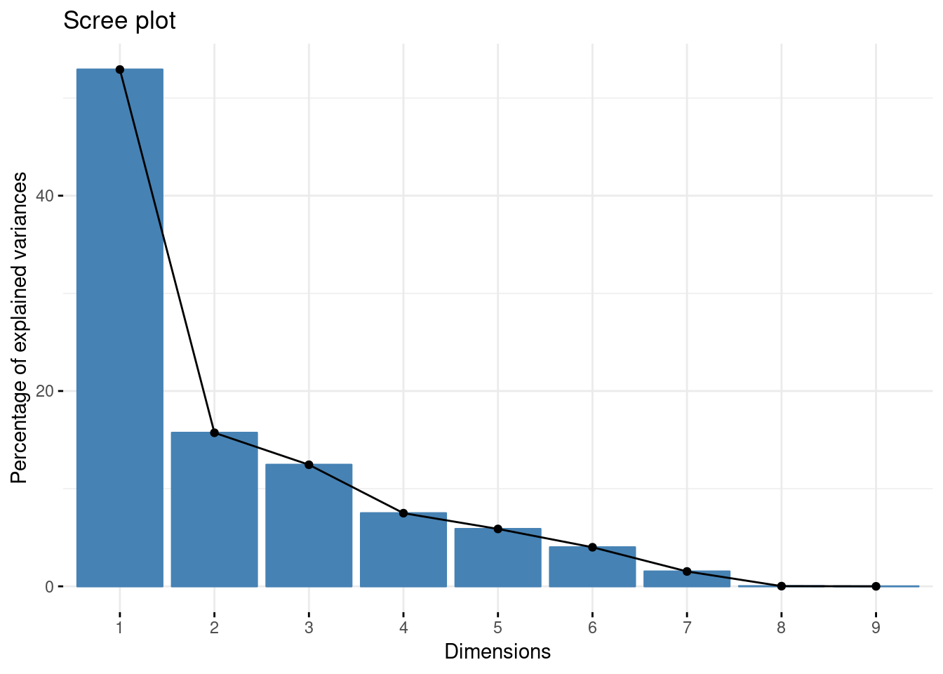
Individuals cloud
- We notice the 1st axis captures 52.9% of the information.
cos2 = rowSums(pca$ind$cos2[ ,1:2] )
fviz_pca_ind(pca, geom = "text" , col.ind = "cos2" ) + scale_color_gradient2( low = "grey" ,mid = "blue" , high = "red" , midpoint = median( cos2) , space = "Lab" )
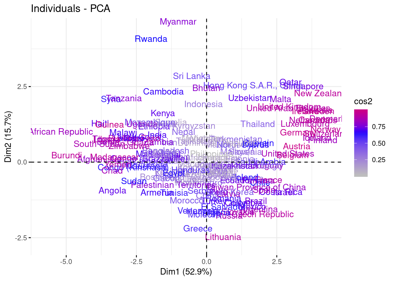
- We notice that the countries of Central-Europe and Eastern-Europe and the countries of Latin-America are very close to the center. So they have an indicator of happiness close to the average.
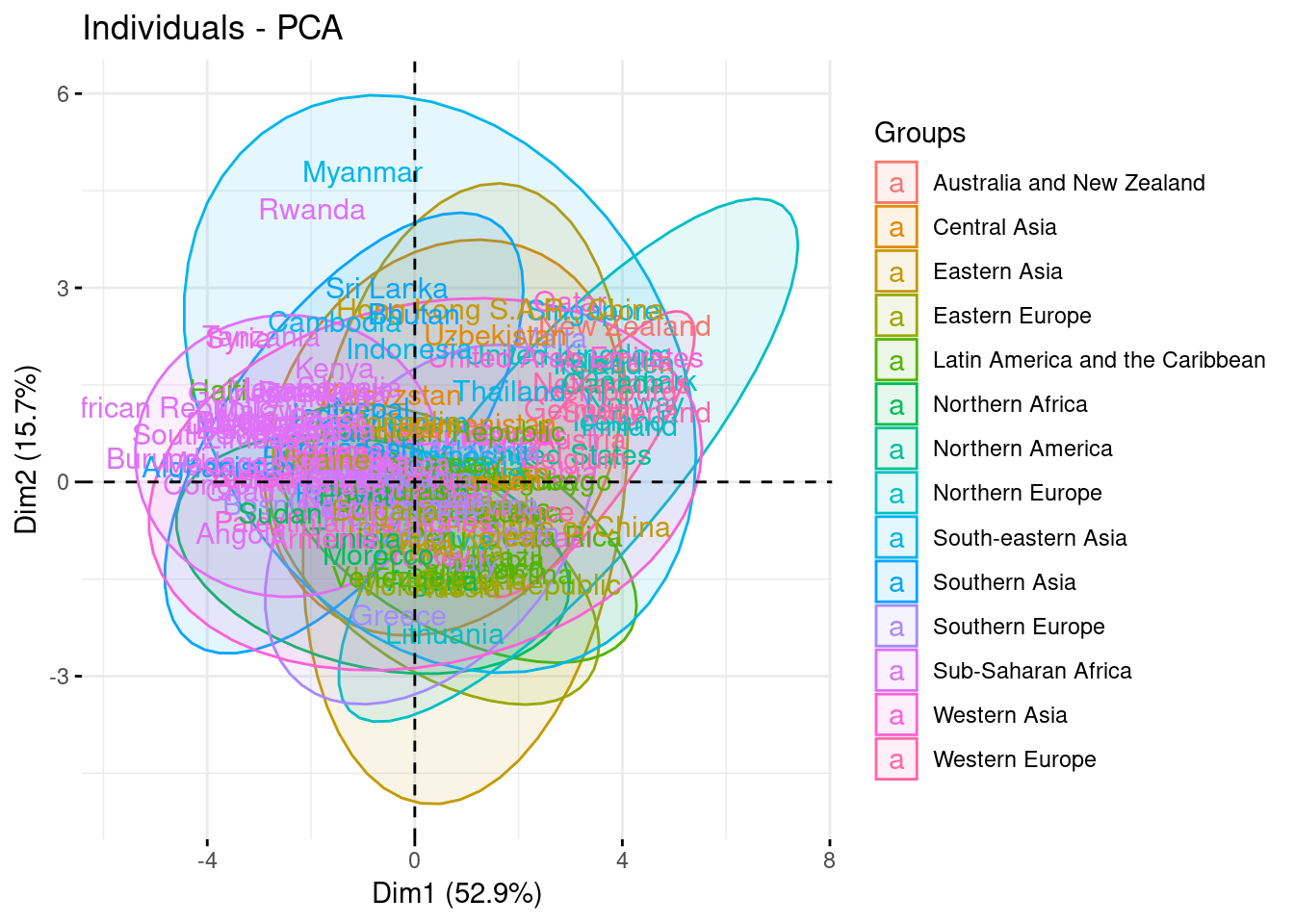
fviz_pca_ind(pca, geom = "text" , habillage = Region, addEllipses = TRUE,ellipse.level =0.95)
## Too few points to calculate an ellipse
## Too few points to calculate an ellipse
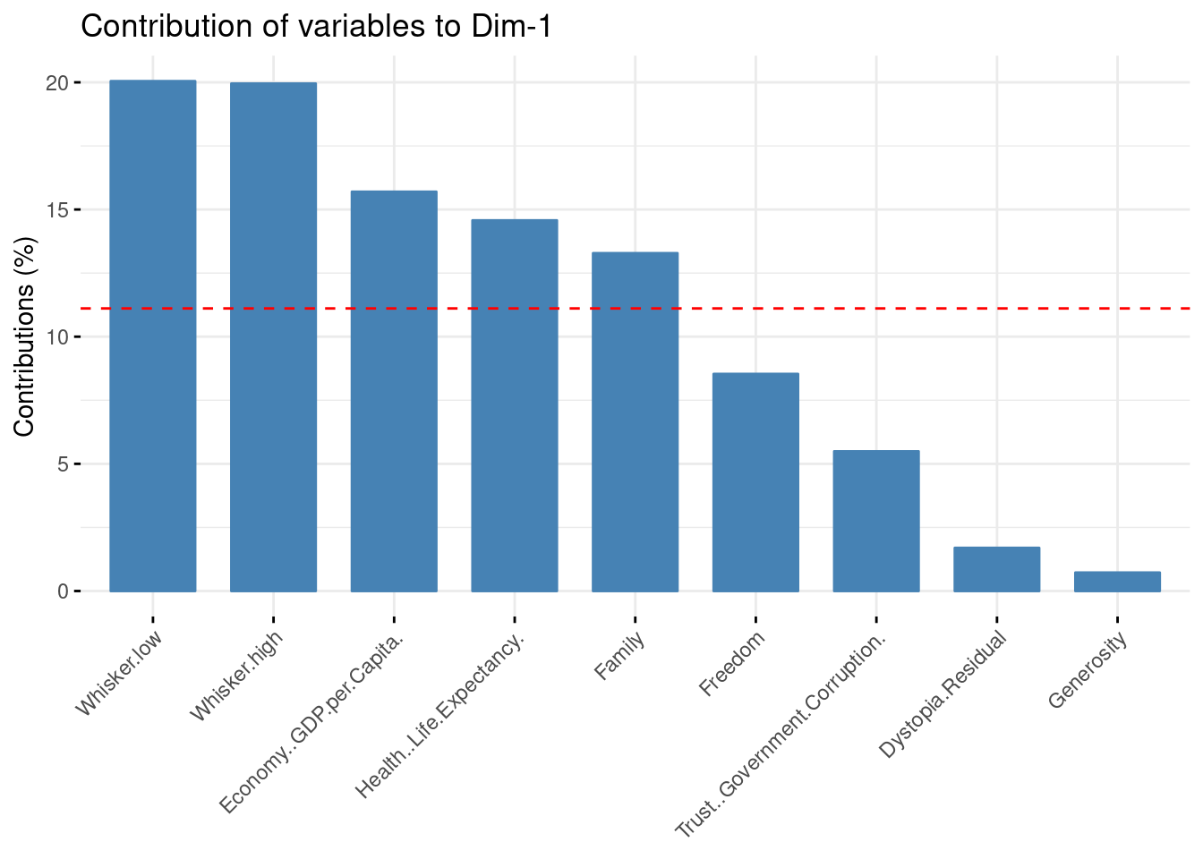
Contribution of the variables in the construction of the first axis.
- “Whisker.high”, “Whisker.low”, “Economy..GDP.per.Capita.”, “Health..Life.Expectancy.” and “Family” contribute the most in the construction of the first axis.
round(sort(pca$var$contrib[,1]),3)
##                    Generosity             Dystopia.Residual
##                         0.725                         1.695
## Trust..Government.Corruption.                       Freedom
##                         5.492                         8.534
##                        Family      Health..Life.Expectancy.
##                        13.283                        14.573
##      Economy..GDP.per.Capita.                  Whisker.high
##                        15.699                        19.952
##                   Whisker.low
##                        20.046
fviz_pca_contrib(pca, choice = "var", axes = 1)
## Warning in fviz_pca_contrib(pca, choice = "var", axes = 1): The function
## fviz_pca_contrib() is deprecated. Please use the function fviz_contrib()
## which can handle outputs of PCA, CA and MCA functions.
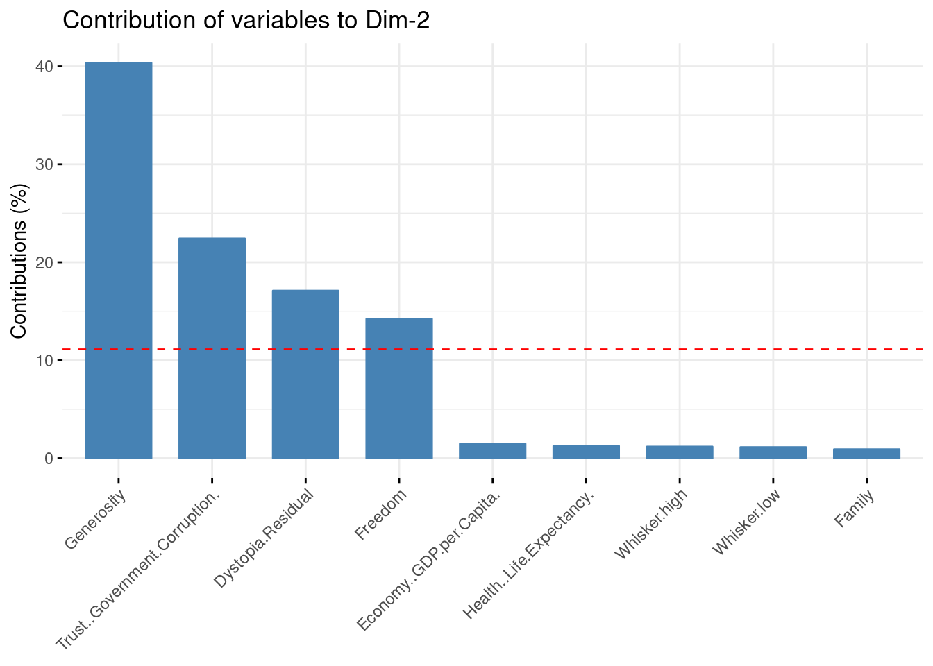
Contribution of the variables in the construction of the second axis.
- “Generosity”,“Trust..Government.Corruption.” ,“Dystopia.Residual” and “Freedom” contribute the most in the construction of the second axis.
round(sort(pca$var$contrib[,2]),3)
##                        Family                   Whisker.low
##                         0.908                         1.123
##                  Whisker.high      Health..Life.Expectancy.
##                         1.176                         1.249
##      Economy..GDP.per.Capita.                       Freedom
##                         1.473                        14.220
##             Dystopia.Residual Trust..Government.Corruption.
##                        17.092                        22.417
##                    Generosity
##                        40.343
fviz_pca_contrib(pca, choice = "var", axes = 2)
## Warning in fviz_pca_contrib(pca, choice = "var", axes = 2): The function
## fviz_pca_contrib() is deprecated. Please use the function fviz_contrib()
## which can handle outputs of PCA, CA and MCA functions.
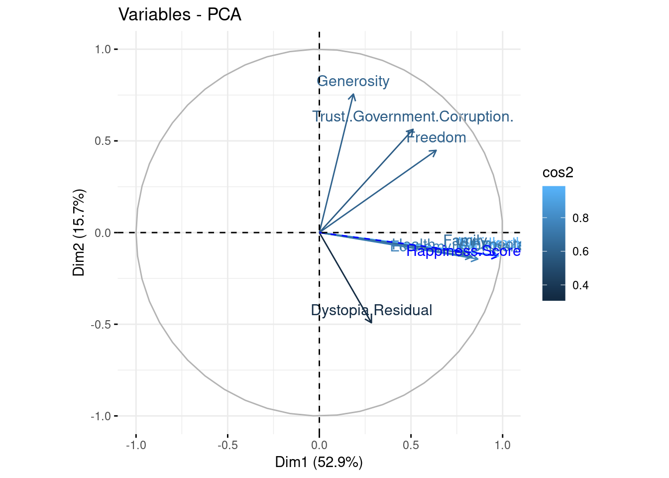
Correlation circle for variables
-
From the circle of correlation, we notice that all the active variables are well represented.
-
The first main component is predominant, it summarizes 52.9% of the total inertia. “Whisker.high”, “Whisker.low”, “Economy..GDP.per.Capita.”, “Health..Life.Expectancy.” and “Family” are strongly correlated with the first axis. They are also positively correlated with “Happiness.Score”. This allows us to conclude that these variables mainly affect the indicator of the happiness of the countries.
-
The second component is relatively important because it summarizes 15.7% of the total inertia.“Generosity”,“Trust..Government.Corruption.” ,“Dystopia.Residual” and “Freedom” are positively correlated with the second axis while the variable “Dystopia.Residual” is negatively correlated with the second axis.
-
fviz_pca_var(pca, geom = c( "text" , "arrow" ) , col.var = "cos2" )
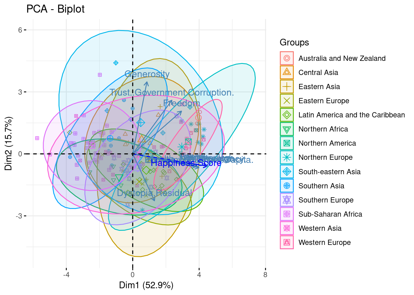
Biplot
-
This graph shows that:
-
The countries of ‘Latin America and Caribbean’ show more generosity and less corruption. According to the variables cloud according to the regions these countries are close to the average happiness score.
-
The countries of ‘Western Europe’ and ‘North America’ have the highest scores of happiness thanks to the social, economic and health indicators.
-
fviz_pca_biplot(pca, label = "var" , habillage = Region, addEllipses = TRUE,ellipse.level = 0.95)
## Too few points to calculate an ellipse
## Too few points to calculate an ellipse
Conclusion
-
Indicators that largely affect a country’s ranking are :
-
‘technical’ based primarily on the economy, health and politics.
-
‘moral’ based essentially on ethics and human values.
-